Volumetric Data#

This guide explains how to visualize volumetric data using FiNNpy.

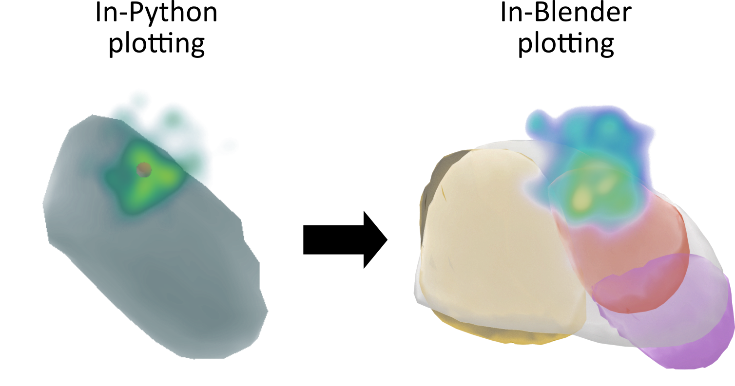
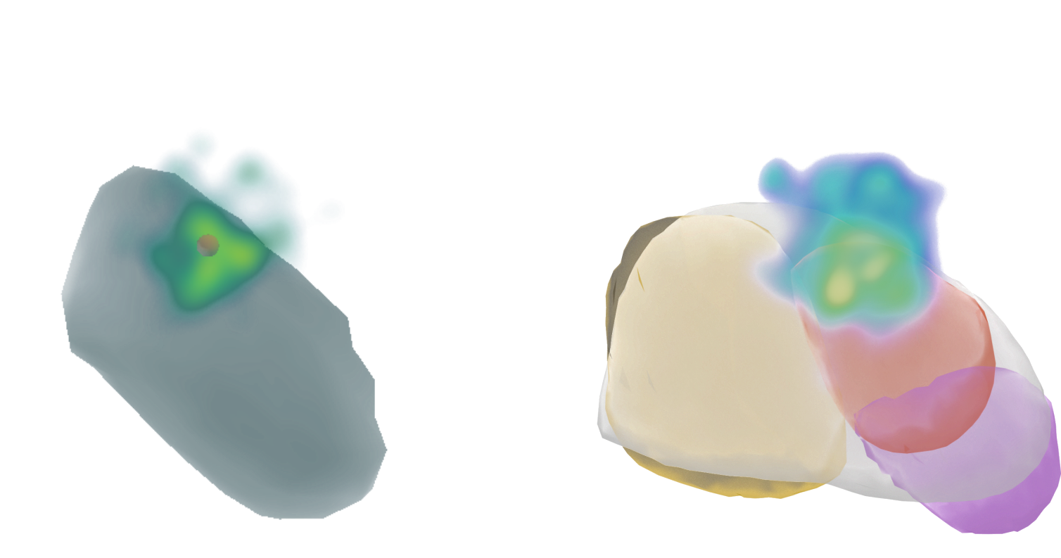
In-Python plotting (left)#

Plotting routines may be imported as follows,

import finnpy.visualization.volumetric_plots as vp

From there, a figure has to be created,

fig = vp.create_figure()

and displayed as follows,

fig.show()

<or>

pv.show_figure(fig)

Several routines are provided to add data to the, as of now, empty plot.

Plot structures#

Structures may be added via

pv.add_structure(fig, path, name, opacity)

fig is the previously created figure.
path is the path to the structure on *.obj format.
name name of the to be added structure.
opacity value of the structure. Defaults to 0.5.

*.obj atlas structures can be extracted as follows (requires 3dslicer; https://www.slicer.org/)

import finnpy.visualization.atlas_nifti_to_obj as anto
anto.conv_ewert(MAT_PATH, NII_PATH, OBJ_PATH, SLICER_PATH)

In case of a permission error, such as below, it is likely that the script needs to be configured as executable.

PermissionError: [Errno 13] Permission denied: '[...]/slicer.sh'

Plot a volume/pointcloud#

Volumes/pointclouds may be added via

pv.add_volume(fig, pts, name, grid_step_cnt, max_filter_sz, gaussian_filter_sigma, opacity)

fig is the previously created figure.
pts are the source datapoints. These need to be a list of 4 valued points (x, y, z, and weight/color).
name name of the to be added structure.
grid_step_cnt resolution of the mesh grid within which the point cloud is computed.
max_filter_sz size of the employed max_filter.
gaussian_filter_sigma size of the employed Gaussian.
opacity value of the structure. Defaults to 0.5.

Points of a volume/pointcloud are projected into a mesh. The size of this mesh is defined by the respective minima/maxima across all axes. The resolution of the mesh can be manually defined. To compensate for potential sparsity from a high resolution, a max filter may be applied to increase the space a single point takes (disabled if max_filter_sz is zero). A Gaussian filter may be applied to smoothen the plot (disabled if gaussian_filter_sigma is zero).

Plot a add_polygon#

Polygons may be added via

add_polygon(fig, pts, faces, name, opacity)

fig is the previously created figure.
pts are the vertices defining the polygon.
faces define which vertices are connected to span surfaces. The required format is either shape(face_cnt, vtx_cnt) or shape(face_cnt * (vtx_cnt + 1),).
name name of the to be added structure.
opacity value of the structure. Defaults to 0.5.

Black background#

The background may be set to black via

set_black_background(fig)

fig is the previously created figure

Add axes#

Axes may be added via

add_axes(fig)

fig is the previously created figure

In-Blender plotting (right)#

To export a figure into blender, it needs to be fully populated (i.e. volumes and other elements added), but not yet displayed, as this clears the figure upon closing.

The following additional software is required for this step:

Blender
FiNNpy’s vti to vtb converter (only for volumes)

How to compile the vti to vtb converter library is explained in Exporting Volumetric Plots to Blender.

The export may be performed via

export_to_blender(structs, volumes, vti_vtb_converter, path = None)

structs List of structures to export. These are returned from the previous calls too add_structure() or add_polygon.
volumes List of volumes to export. These are returned from previous calls to add_volume().
vti_vtb_converter Path to the vti_to_vtb converter library.
outpath Path to save the files which will be imported into blender.

This function iterates through all provides structures and volumes, creating a blender-readable file for each. Subsequently, this may be imported into blender.

FiNNPY