Directional absolute coherence

This function may be called for data in the time domain, the frequency domain, or (if correctly aligned) in the complex coherency domain.

Note

Use the following function for time domain data.

Note

Use the following function for frequency domain data.

Note

Use the following function for complex coherency domain data.

The following code example shows how to apply directional absolute coherence to measure sfc.

import numpy as np

import matplotlib
matplotlib.use("Qt5agg")
import matplotlib.pyplot as plt

import finn.sfc.td as td
import finn.sfc.fd as fd
import finn.sfc.cd as cohd

import finn.sfc._misc as misc
import demo_data.demo_data_paths as paths

def main():
    data = np.load(paths.fct_sfc_data)
    frequency_sampling = 5500
    frequency_peak = 30

    noise_weight = 0.2

    phase_min = -90
    phase_max = 270
    phase_step = 4

    fmin = 28
    fmax = 33
    nperseg = frequency_sampling
    nfft = frequency_sampling
    return_signed_conn = True
    minimal_angle_thresh = 4

    #Generate data
    offset = int(np.ceil(frequency_sampling/frequency_peak))
    loc_data = data[offset:]
    signal_1 = np.zeros((loc_data).shape)
    signal_1 += loc_data
    signal_1 += np.random.random(len(loc_data)) * noise_weight

    conn_vals = list()
    fig = plt.figure()
    for phase_shift in np.arange(phase_min, phase_max, phase_step):
        loc_offset = offset - int(np.ceil(frequency_sampling/frequency_peak * phase_shift/360))
        loc_data = data[(loc_offset):]
        signal_2 = np.zeros(loc_data.shape)
        signal_2 += loc_data
        signal_2 += np.random.random(len(loc_data)) * noise_weight

        plt.cla()
        plt.plot(signal_1[:500], color = "blue")
        plt.plot(signal_2[:500], color = "red")
        plt.title("Signal shifted by %2.f degree around %2.2fHz" % (float(phase_shift), float(frequency_peak)))
        plt.show(block = False)
        plt.pause(0.001)

        dac_value_td = calc_from_time_domain(signal_1, signal_2, fmin, fmax, frequency_sampling, nperseg, nfft, return_signed_conn, minimal_angle_thresh)
        dac_value_fd = calc_from_time_domain(signal_1, signal_2, fmin, fmax, frequency_sampling, nperseg, nfft, return_signed_conn, minimal_angle_thresh)
        dac_value_coh = calc_from_time_domain(signal_1, signal_2, fmin, fmax, frequency_sampling, nperseg, nfft, return_signed_conn, minimal_angle_thresh)

        if (np.isnan(dac_value_td) == False and np.isnan(dac_value_fd) == False and np.isnan(dac_value_coh) == False):
            if (dac_value_td != dac_value_fd or dac_value_td != dac_value_coh):
                print("Error")

        conn_vals.append(dac_value_td if (np.isnan(dac_value_td) == False) else 0)

    plt.close(fig)

    plt.figure()
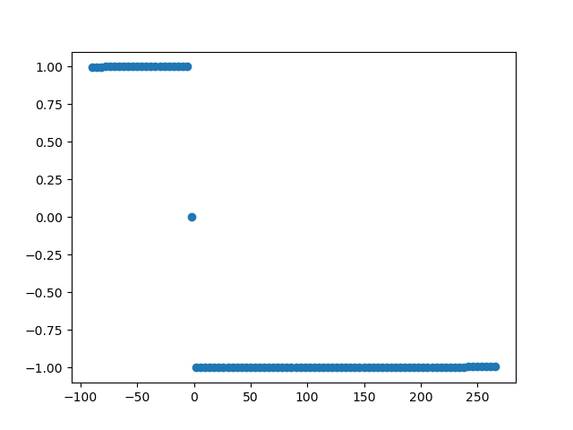
    plt.scatter(np.arange(phase_min, phase_max, phase_step), conn_vals)
    plt.show(block = True)


def calc_from_time_domain(signal_1, signal_2, fmin, fmax, frequency_sampling, nperseg, nfft, return_signed_conn, minimal_angle_thresh):
    return td.run_dac(signal_1, signal_2, fmin , fmax, frequency_sampling, nperseg, nfft, return_signed_conn, minimal_angle_thresh)[1]

def calc_from_frequency_domain(signal_1, signal_2, fmin, fmax, frequency_sampling, nperseg, nfft, return_signed_conn, minimal_angle_thresh):
    seg_data_X = misc._segment_data(signal_1, nperseg, pad_type = "zero")
    seg_data_Y = misc._segment_data(signal_2, nperseg, pad_type = "zero")

    (bins, fd_signal_1) = misc._calc_FFT(seg_data_X, frequency_sampling, nfft, window = "hanning")
    (_,    fd_signal_2) = misc._calc_FFT(seg_data_Y, frequency_sampling, nfft, window = "hanning")

    return fd.run_dac(fd_signal_1, fd_signal_2, bins, fmin, fmax, return_signed_conn, minimal_angle_thresh)[1]

def calc_from_coherency_domain(signal_1, signal_2, fmin, fmax, frequency_sampling, nperseg, nfft, return_signed_conn, minimal_angle_thresh):
    (bins, coh) = td.run_cc(signal_1, signal_2, nperseg, "zero", frequency_sampling, nfft, "hanning")

    return cohd.run_dac(coh, bins, fmin, fmax, return_signed_conn, minimal_angle_thresh)[1]


main()

Shifting the reference signal from -90° to + 270° emulates connectivity in different directions and volume conductance at 0°. Ordinarily volume conduction is returned as nan, however in the scope of this example it is returned as 0.