Bad channel identification

cleansing.bad_channel_identification.run(data, ch_names, fs, ref_areas=[[105, 120], [135, 145], [155, 195]], broadness=3, visual_inspection=True)

Identifies which channels have substantially more or less power in the frequency ranges defined by ref_areas. Channels whose power is more different than broadness (default: 3) standard deviations will be primed as faulty channels. In case visual inspection is active (default: True), the automatic results can be further refined via manual selection.

Attention: Function is parallelized. Sensitive parts are placed within a locked area to avoid unexpected behaviour.

Parameters:

• data – Input data in the format channel x samples.

• ch_names – Names of the channels. Used for visualization purposes only. Order has to match the channel order of data.

• fs – List of sampling frequencies for each channel.

• ref_areas – Spectral reference areas used for power estimation. Only power within these ranges is defined. It is recommended to choose ranges, which are not part of any evaluation to decrease the chances of pre-processing induced biases.

• broadness – Number of standard deviations threshold by which channels are automatically categorized as faulty. In case visual inspection is enabled (recommended) this only results in priming the channels.

• visual_inspection – Toggles visual inspection on and off.

Returns:

(valid_list, invalid_list, score). List of valid channels, invalid channels and their respective z-scores.

The following code example shows how to apply bad channel identification & subsequent restoration.

import numpy as np
import random

import matplotlib
matplotlib.use("Qt5agg")
import matplotlib.pyplot as plt

import finn.cleansing.bad_channel_identification as bci
import finn.cleansing.channel_restoration as cr

def main():
    #Configure sample data
    channel_count = 64
    frequency = [random.randint(5, 50) for _ in range(channel_count)]
    data_range = np.arange(0, 10000)
    frequency_sampling = 200
    ch_names = ['O1', 'Oz', 'O2', 'PO9', 'PO7', 'PO3', 'POz', 'PO4', 'PO8', 'PO10', 'P9', 'P7', 'P5', 'P3', 'P1', 'Pz', 'P2', 'P4', 'P6', 'P8', 'P10',
               'TP9', 'TP7', 'CP5', 'CP3', 'CP1', 'CPz', 'CP2', 'CP4', 'CP6', 'TP8', 'TP10', 'T9', 'T7', 'C5', 'C3', 'C1', 'Cz', 'C2', 'C4', 'C6', 'T8', 'T10',
               'FT9', 'FT7', 'FC5', 'FC3', 'FC1', 'FCz', 'FC2', 'FC4', 'FC6', 'FT8', 'FT10', 'F9', 'F7', 'F5', 'F3', 'F1', 'Fz', 'F2', 'F4', 'F6', 'F8', 'F10',
               'AF9', 'AF7', 'AF3', 'AFz', 'AF4', 'AF8', 'AF10', 'Fp1', 'Fpz', 'Fp2']

    #Configure noise data
    frequency_noise = 50
    shared_noise_strength = 1
    random_noise_strength = 1

    #Configure bad channel
    bad_channel_idx = 1
    bad_channel_signal_power = 1.1

    #Generate some sample data
    raw_data = [None for _ in range(channel_count)]
    for channel_idx in range(channel_count):
        genuine_signal = np.sin(2 * np.pi * frequency[channel_idx] * data_range / frequency_sampling)
        shared_noise_signal = np.sin(2 * np.pi * frequency_noise * data_range / frequency_sampling) * shared_noise_strength
        random_noise_signal = np.random.random(len(data_range)) * random_noise_strength

        raw_data[channel_idx] = genuine_signal + shared_noise_signal + random_noise_signal

    raw_data[bad_channel_idx] = np.random.random(len(data_range)) * bad_channel_signal_power
    #raw_data = np.asarray(raw_data)

    #Faulty channel gets identified
    (_, invalid_list, _) = bci.run(raw_data, ch_names, [frequency_sampling for _ in range(channel_count)], [[60, 100]], broadness = 3, visual_inspection = True)
    #Faulty channel gets substituted via neighbors
    rest_data = cr.run(raw_data, ch_names, invalid_list)

    #visualization
    channels_to_plot = 3
    (_, axes) = plt.subplots(channels_to_plot, 2)
    for channel_idx in range(channels_to_plot):
        axes[channel_idx, 0].plot(raw_data[channel_idx][:200])
        axes[channel_idx, 1].plot(rest_data[channel_idx][:200])

    axes[0, 0].set_title("before correction")
    axes[0, 1].set_title("after correction")

    axes[0, 0].set_ylabel("Channel #0\n"); axes[0, 0].set_yticks([-2, 0, 2])
    axes[1, 0].set_ylabel("Channel #1\n(faulty channel)"); axes[1, 0].set_yticks([-2, 0, 2])
    axes[2, 0].set_ylabel("Channel #2\n"); axes[2, 0].set_yticks([-2, 0, 2])

    plt.show()

main()

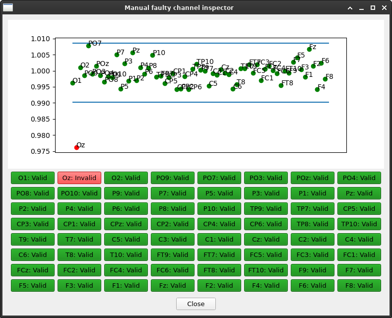
Applying bad channel identification automatically selected channels whose broadband power is more than two standard deviations different from other channels. Yet, manual optimization of the selection is possible (and recommended). Manual adjustments can be performed in the screen below.